Cambrian ecosystems

This session is a workshop exploring Cambrian ecosystems, designed to help you to revise concepts from earlier in the course, and guide your approach to the Wenlock assignment.

It's a little different to previous sessions: the focus is on developing your interpretation and critical thinking skills, so we'll be working through the content in groups. The online material duplicates what we will cover in the classroom, but is provided here to allow you to spend additional time grappling with the concepts – and pondering how they might be applied to your Wenlock project.

As such there's no explicit preparation for the session, but you may wish to watch the refresher on the Cambrian Explosion (embedded below). Perhaps you could use the time gained to progress your Wenlock data analysis.
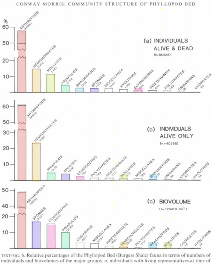
Credit: Rob Nicholls, Palaeocreations

The Cambrian Fauna

The birth of animal complexity

The Cambrian “explosion” marked the sudden onset of complex animal-dominated ecosystems, and the origin of the modern animal groups, in a geologically brief window of time.

Was there something special about the Cambrian that precipitated this rapid radiation – or does this evolutionary event only stand out from others because there was so little there before it?

This is the focus of my own research. Today we're going to look in some depth at a Cambrian community.

Clueless about the Cambrian? Catch up with this optional refresher video, which will set the scene for this session.

The Cambrian Fauna

In a seminal palaeontological study, Jack Sepkoski showed that a ‘Cambrian fauna’ (marked I in figure) with a distinctive taxonomic composition arose in this period, before waning almost immediately during the Ordovician radiation.

Sepkoski compiled a database of the stratigraphic occurrence of marine families, allowing the first detailed analysis of the diversity of each invertebrate class (the Linnean rank below a phylum) through time. Elegant statistical analysis showed, remarkably, that the diversity of each class could be described as a blending of three ‘fundamental trends’ (factors).

Blending these three factors together accounts for the vast majority (>90%) of the pattern of diversity through time; the residuals largely correspond to times of mass extinction or rapid diversification.

Some classes’ trends (e.g. Trilobites, articulate brachiopods, gastropod molluscs) map almost exactly onto one of the three factors – these groups are considered to represent a ‘Cambrian’, ‘Palaeozoic’ and ‘Recent’ fauna. Other groups (e.g. ostracod arthropods, corals) represent a blending of two or three factors.

  • Which factors blend to account for the diversity of corals (Anthozoa, rightmost column) through time?
  • Factor I
  • Factor II
  • Factor III
  • Many classes map to a single factor (find some examples). Why might corals represent a blending of two?

Characterizing the faunas

Sepkoski suggested that members the three different faunas might be characterised by different evolutionary parameters. We’re going to explore this now with an ecological analogy. Could the Precambrian oceans, essentially devoid of macroscopic life, be analogous to a patch of ground recently cleared and about to undergo ecological succession? If so, the first animal species to evolve in the Cambrian might have something in common with the first individuals to arrive on a patch of new earth.

Let’s refresh our memory of succession. Imagine that a nettle seed, a hawthorn berry, and an acorn (oak seed) germinate on a patch of bare earth. In the left-hand plot, draw three curves, corresponding to the population size of each population (of nettles, hawthorn shrubs, and oak trees). In the right-hand plot, stack these curves vertically to depict the proportion of individuals that are (i), nettles; (ii), hawthorns; (iii) oaks.

  • Double-click here to show my approximate answer.

Developing the analogy

Let’s pretend for a moment that families, each containing many species, come to fill empty ecospace over evolutionary timescales in the same way that populations, each containing many individuals, come to fill empty ecospace over ecological timescales.

Let’s explore this analogy further (without worrying, yet, whether it is a good analogy). Complete this table:

Ecological succession Evolutionary analogue Hint
Population of individuals Family of species
Birth of new individual 🖉_______ of a new species
Death of an individual 🖉_______ of a species
Reproductive rate 🖉_______ rate
Death rate 🖉_______ rate
Life expectancy 🖉_______

Remind yourself of the trajectories of the Cambrian (I), Palæozoic (II) and Recent (III) faunas in Sepkoski's diversity plot.

Assuming that the analogy with ecological succession holds true, infer the properties of each fauna:

Cambrian Fauna (I) Palæozoic Fauna (II) Recent Fauna (III)
Speciation rate 🖉high / medium / low high / medium / low high / medium / low
Species longevity 🖉high / medium / low high / medium / low high / medium / low
Competitivity 🖉high / medium / low high / medium / low high / medium / low
  • If you get stuck, come back to this table later.
  • In an ecological context, what sort of life strategy is associated with the lifespan and reproductive rate you reconstructed for the Cambrian and Recent faunas?
  • What other characteristics do you associate with these life strategies?
  • Assuming that the analogy with succession holds, what characteristics would you predict might characterise (i), the Cambrian fauna; (ii), the Recent fauna?

As it happens, the predictions of our ‘succession analogy’ are not too wide of the mark. In particular, the Cambrian is often viewed as 'less competitive' than later periods, conjuring a harmonic idyll in which predation only exerted a secondary influence on ecosystem structure.

This raises an interesting question: do we need to invoke large-scale macroevolutionary processes to explain the replacement of biotas and the pattern of diversity through time, or do the first-order patterns in biodiversity simply represent the null expectation as life gradually conquers an uninhabited realm?

Credit: Martin R. Smith / Royal Ontario Museum

The Burgess Shale

A case study of a Cambrian community

Preservation

The Burgess Shale is an exceptional fossil deposit that offers an unrivalled glimpse into Cambrian ecology. Event beds, packed with fossilized 'soft' anatomy, range from 2–200 mm thick, separated by fossil-poor background sedimentation; each corresponds to a single obrution event.

As always, it's worth worrying to what extent the fossil assemblage is representative of the living community, and to what extent the living community was representative of Cambrian communities more generally.

  • What factors make the Burgess Shale promising for ecological study?
  • Is it legitimate to draw conclusions about Cambrian communities in general from the Burgess Shale?
  • How is the taxonomic composition of fossil assemblages likely to relate to that of the original (live) communities? What biases might be in play – and how might we evaluate their effects?

Awesome Resources

How to count the data

We're going to look at data from two studies: Conway Morris 1986, which uses ‘familiar’ techniques on ‘old’ collections, which incorporate talus material and were not collected systematically (anything dubbed inferior was chucked down the hillside); and Caron & Jackson 2008, which performs a bed-by-bed analysis and some more sophisticated stats for additional insight.

Conway Morris takes three different counts: all individuals; living individuals only (e.g. discounting empty shells); and biovolume. These results differ in certain respects (see figure).

Explain the following trends:

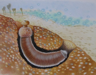
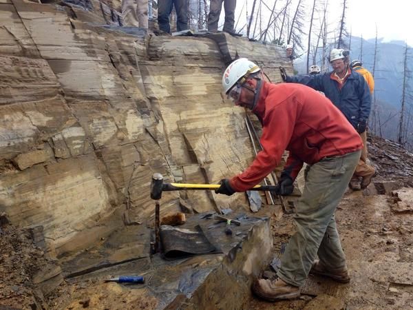
Systematic sampling allows Caron (foreground) to link samples to specific horizons.
  • Super-abundant in all ways of counting (arthropods)
  • Many individuals, little biovolume (hemichordates)
  • Few individuals, much biovolume (e.g. sponges)
  • Many individuals, few live individuals (molluscs, brachiopods)
  • Consistently in the middle (priapulid worms)

Habitat and feeding

Trends in habitat and feeding habit also vary depending on counting mechanism – but some observations are robust to this.

Use the slides below to interpret the ecology of the Burgess Shale. (Advance the slides to colour-code the habits.)

  • Habitat bars are ordered from ‘more to less active’ from left to right; feeding habit categories are DC, DS: Deposit; SU: Suspension; PC: Predator / carnivore / scavenger.
  • Not loading? Log in to a Microsoft website (Outlook?) using your Durham account, or open in a separate tab.
  • How does the mode of counting influence the patterns in life habits (habitat)?
  • Did predators play an important role in Cambrian ecosystems?

Use the percentage data to (approximately) plot the Burgess Shale assemblage on Scott's (1978) ternary diagrams of Cenozoic environments.

  • Does the composition of individuals in the Burgess Shale correspond to the distribution of habitats and feeding habits in a Cenozoic marine ecosystem? Account for any differences.

The trophic nucleus

The trophic nucleus (remind yourself of the definition…) gives a quick-and-dirty overview of the dominant consituents of an ecosystem.

  • Use the trophic nucleus (below) to discuss the prevalance of predation in Cambrian ecosystems.
Miniature Marrella (~10 mm long)
Credit: Cédric Aria

Bed-by-bed analysis

Digging deeper

We've now got an overall picture of the Burgess Shale community though bulk analysis of all its inhabitants. But do these trends over the ‘averaged’ data across the entire Phyllopod bed truly represent individual living communities?

The ‘core species’ (defined, ad hoc, as 5 most abundant) are pretty consistent from bed to bed. So is evenness and diversity (species richness), with the occasional outlier.

  • What are the strengths and limitations of the 'core species' approach?

Coordination analysis

The table suggests that some beds are more similar than others. Coordination analysis allows such differences to be picked apart. (See Caron & Jackson 2008 for details of the analysis.)

  • Why might certain species consistently occur together?
  • Reconcile your suggestions with the evenness and richness trends through the bedding assemblages.

Whittaker (rank-abundance) plots

Analyses of the whole Burgess Shale assemblage, and of individual beds, and of individual niches all fit a log-normal distribution best (with the odd exception – but run enough tests and you’ll always find an odd one out!).

  • Provide an ecological interpretation of this log-normal distribution
Credit: Martin R. Smith / Smithsonian

Bringing it together

Conclusions for the Cambrian

Now bring together all the aspects we’ve addressed today. If you've been working in a group, see whether you agree on the following points:

  • To what extent was the Burgess Shale a ‘typical’ Cambrian community?
  • What were the ecological properties of the Burgess Shale life assemblage? In what environment did its denizens live?
  • How is the Burgess Shale (and Cambrian ecosystems more generally?) similar to and different from modern ecosystems?

Linking to the Wenlock

You now have slab-by-slab data for the whole class, and have hopefully started to ponder how to approach the analysis.

How might you apply the ideas discussed today, in combination with the techniques introduced in the first two sessions? Here are some questions you might think about:

  • How might you characterize the fauna of the Wenlock biota as a whole?
    • What is its trophic nucleus?
    • What feeding habits and substrate niches predominate?
    • What does this tell you about the environment in which the fauna lived?
  • Is each group’s sample simply a microcosm of the biota as a whole?
    • Do any slabs stand out as having a distinct taxonomic or ecological composition?
    • Do slabs generally have the same diversity and dominance? What accounts for any exceptions?
    • What does this tell you about the environment in which the organisms lived?
  • How might the collected data differ from the original life assemblage?
    • What is the direction and extent of any biases you can identify?
    • If these potential biases are extensive, how would they affect your interpretation?
    • Are you able to quantify or correct for these biases? If not, what caveats should be raised when you discuss your results?

Take the opportuntity to chat with a demonstrator today to be confident in how you will approach any of these questions that you feel might be relevant – and any other questions that might occur to you. Make a start on some of the analyses as soon as you can.

I would suggest conducting your analyses this week. Next week you can discuss your interpretations, and get help on any analyses that proved intransigent. That’ll give you a week to finish writing up your results, before receiving feedback on your draft submission.

Credit: Sedgwick Museum

Suggestions for further reading

  • * Conway Morris, S. (1986). The community structure of the Middle Cambrian Phyllopod Bed (Burgess Shale). Palaeontology, 29(3), 423–467.
  • Sepkoski, J. J. (1981). A Factor Analytic Description of the Phanerozoic Marine Fossil Record. Paleobiology, 7, 36–53.
  • Caron, J.-B., & Jackson, D. A. (2008). Paleoecology of the Greater Phyllopod Bed community, Burgess Shale. Palaeogeography, Palaeoclimatology, Palaeoecology, 258(3), 222–256.
  • Caron, J.-B., & Jackson, D. A. (2006). Taphonomy of the Greater Phyllopod Bed community, Burgess Shale. Palaios, 21, 451–465.
  • Now might also be a good time to refer back to your notes on previous sessions, particularly those on Palaeoecology and Succession.