Success! Another week's content complete.
Use the "Ask" button to propose questions or topics we should cover in our face-to-face session. Give questions you'd like addressed the "thumbs up".
Session 2: Life Histories and Succession
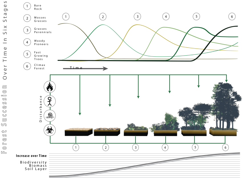
In the previous session we explored the types of places where diversity might be high or low. This time we will see how diversity might change at a single location as empty ecospace is colonized, on ecological timescales (years to centuries).
Distinguish r-selected and K-selected species
Understand the principle of ecological succession, and its application to the fossil record
Relate the diversity and composition of fossil assemblages to their depositional environment
Over the course of a number of years, any fresh environment will rapidly be colonized by generalist taxa with a high dispersal rate that can grow rapidly in any environment. Eventually, specialists that are better adapted to that environment will gradually arrive, ultimately displacing the original generalists.
Note that these timescales are too short for evolution to be a significant factor. We’ll explore how the character of ecosystems has changed over geological time (millions of years) later in the course.
Two approaches to life: meeting r- and K-strategists
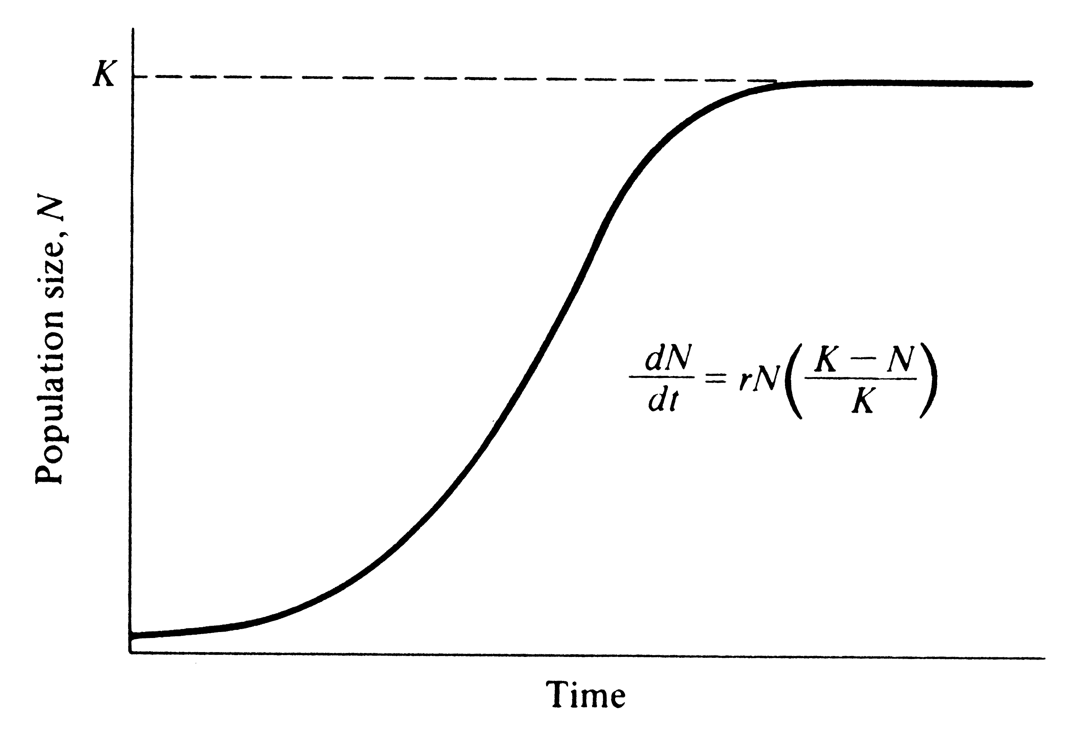
Rapidly-dispersing generalists can be discriminated mathematically from slow-and-steady specialist competitors based on the formula

where:
The equation can be expressed verbally as:
The change in the number of individuals per unit time (dN/dt) is equal to the number of offspring per individual (r), multiplied by the number of individuals (N), multiplied by the proportion of the carrying capacity that is unoccupied (K − N / K).
The equation predicts that the population of an environment will grow exponentially until it approaches the carrying capacity, at which point it will level off.
When an environment is empty (perhaps a storm deposit has just smothered the pre-existing community), the value of r is the dominant control on population size.
| Why? | if | N ≪ K, |
| then | K − N ≈ K, | |
| so | (K − N) / K ≈ 1 | |
| and | dN/dt ≈ rN. |
When an environment is ‘full’ (N ≈ K), conversely, the population size is controlled by the value of K; successful taxa are those that can best compete for the resources that limit carrying capacity.
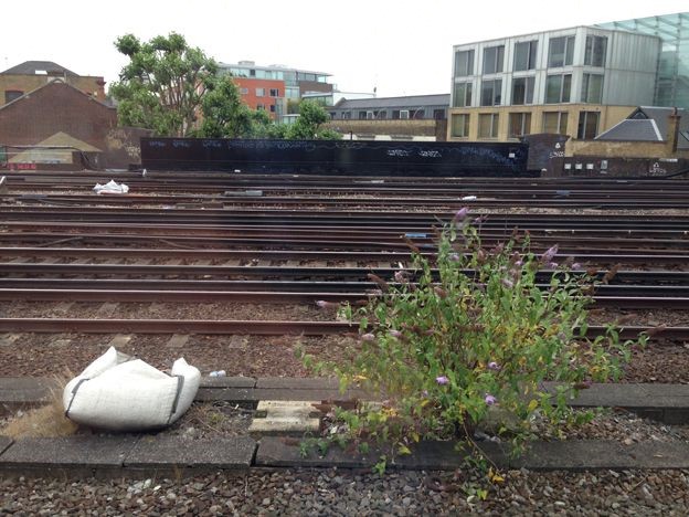
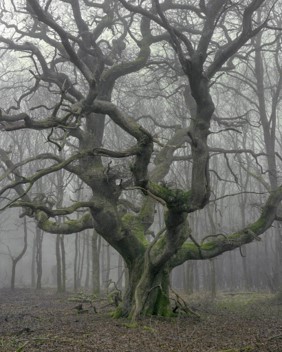
On this basis, one might distinguish two biological strategies. One strategy, the r-strategy, is to make sure that you are the first on the scene, and can reproduce rapidly once you get there (i.e. have a big r). Then you’ll quickly rise to dominance. The opposite strategy, the K-strategy, is to play the long game, and be a good competitor; it might take you longer to get a foothold, but when population size is limited by K rather than r, you will be better suited to compete for the resource that is limiting the carrying capacity. Next time you take a train journey, you’ll notice r-strategists (silver birch, buddleia) colonizing disused sidings and abandoned platforms, whilst K-strategists (holly, oaks) typify ancient woodland that’s had plenty of time to mature.
| r-strategists | K-strategists |
|---|---|
|
|
An age-frequency curve plots the relative frequency of individuals of a certain age in death assemblages. Pragmatically, it's usually much easier to measure a dead organism's size than to calculate its age, so you'll typically see size-frequency plots as a proxy.
A survivorship curve is another way of depicting the life history of a species. Survivorship rate plummets rapidly in taxa with high infant mortality, but individuals that survive to adulthood can expect a long life ahead (Type III). Taxa in which the probability of survival is independent of age sit along a linear Type II curve. Taxa in which most juveniles survive to adulthood sit upon a Type I curve.

You've learned a lot of new concepts so far. Why not make yourself a coffee and watch Sir David expound the life cycle of corals (a group with a magnificent fossil record)?
Once you're done, draw a size-frequency (or age-frequency) and survivorship curve for this coral species.
Large numbers of tiny offspring with a tiny chance of survival, looking for fresh, uncolonized sites at an early stage of succession to occupy? Hopefully you recognized this as an excellent example of r-selection at work.
Your size-frequency and survivorship plots should look similar to those you drew for r-selected species above.
Let's recap what we've learned so far, with our sedimentary environments hat on – remember, we are interested in what we can learn about original habitat based on our ecological observations.

Pioneer communities are typically dominated by a low diversity of r-strategists, whereas climax communities usually host a more diverse suite of K-strategists.
As such, pioneer communities typically have a small trophic nucleus (the majority of individuals belong to just one or two species that boast a very high reproductive rate), whereas climax communities have a larger trophic nucleus incorporating a wide variety of specialists.

Pioneer and climax communities also differ in two different aspects of diversity:
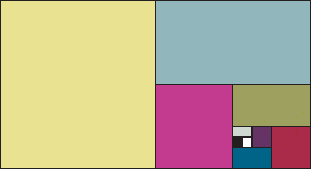
The stacked bar charts on the right depict two communities: each block represents a separate species; larger blocks contain more individuals.
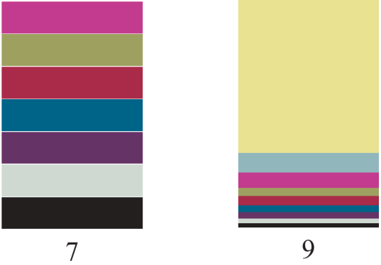
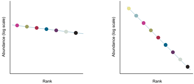
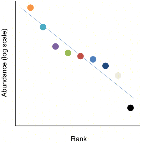
A rank-abundance plot (sometimes called a Whittaker plot) shows how diversity is spread between species. It's a more sophisticated way of depicting species richness alongside dominance. Taxa are ordered by the number of observed individuals, with the rank order plotted on the x axis, and the logarithm of the number of individuals plotted on the y axis.
Use the two rank-abundance plots to answer the following questions:
With me so far? Things get a bit more complicated with octave plots. These are very useful, and enhance the degree and sophistication of analysis that you can attempt: but if you're already starting to feel out of your mathematical depth, then you should be able to get by without them.
An octave plot is a histogram that provides an indication of how many species are high, low, or intermediate diversity. As with any histogram, the y axis denotes frequency; unusually, however, the x-axis is log transformed, such that the lower bound of each interval (‘octave’) is twice the lower bound of the last (by analogy with the frequencies of a musical scale). The first bar thus shows the number of taxa known from only one individual, the next bar, the number of taxa known from 2–3 individuals, then subsequent bars from 4–7, 8–15, 16–31, individuals.

A straight line on a rank-abundance plot fits with a geometric model of species diversity. One way of visualizing this model is to imagine that the first species to arrive consumes a given proportion (half, perhaps) of the available resources. The next species to arrive consumes the same proportion of the remaining resources, and so on for each species. When ordered, each species thus contains a half (or whatever fraction characterizes that assemblage) of the biomass as the next most abundant species. The slope of the line determines what proportion of the ‘remaining’ resources each species consumes; a shallow slope indicates that resources are spread more evenly between species, indicating a more diverse community. The geometric model applies well to ecosystems in the early stages of succession, or in stressed environments.
An alternative model of species diversity is the log-normal model. This model produces an S-shape on a rank-abundance plot: only a few species are very abundant or very rare; the majority of species are intermediate in abundance. When plotted on an octave plot, a population with a log-normal diversity distribution produces a bell-shaped curve – though because taxa known from fewer than one individual are not observed, the left-hand side of the bell curve will be truncated in small sample sizes.
Let's recap what we've learned so far, with our sedimentary environments hat on – remember, we are interested in what we can learn about original habitat based on our ecological observations.

Diversity is maximised when an environment is intermittently disturbed
Maximum diversity is thought to be maintained when an environment is intermittently disturbed, allowing the co-existence of r- and K- strategists.
Success! Another week's content complete.
Use the "Ask" button to propose questions or topics we should cover in our face-to-face session. Give questions you'd like addressed the "thumbs up".
Key concepts:
or
For more depth: